Simulating the Vicsek Model (with time delay) - How do birds flock and insects swarm

In two previous posts we got to know two main things:

We can analyse the behaviour of groups of animals using statistical tools like correlation functions
We can simulate this behaviour using for example the Vicsek model, and by analysing it the same way as natural groups we can measure the accurateness of the model in replicating natural phenomena.

We also learned that the standard Vicsek model suffers from one weakness: it lacks an inertial term, which seems to be important in imitating the behaviour of biological systems. So the goal of this post will be to figure out a way to simulate the Vicsek model with time delay. Let's start by

Analysing the equations of motion

\vec{v_i}(t+1) = v_{0}\mathscr{R}_{\eta}\Theta \left[ \vec{v_i}(t) + \sum_{ j \neq i }{ n_{ij} \vec{v_j}(t) } \right] ,

\vec{r_i}(t+1) = \vec{r_i}(t) + \vec{v_i}(t+1) .

So what do we see here? The first main thing to realise is that the first equation signifies calculation of velocity for the next point in time (call it second for example), and the second one is calculating the position $\vec{r}$ for that next point in time. They are both vectors, since we want to generalise these equations to any number of dimensions we're interested in (we'll work in 3D). The index in $\vec{v_i}$ and $\vec{r_i}$ signify the index of the member in our group of particles. So we have the left hand side of both equations figured out. As you can see, the model is indeed very simple - just two equations for two things we need to keep track of - position and velocity. We don't even deal directly with accelerations (kind of, implicitly). Eighth grade physics, right?

Now let's have a look at the right hand side. Let's start with the obviously easier one - the position equation (second one). All it says is that the position of particle $i$ at the next time step $t+1$ is equal to the position of the particle at the current time step $t$ plus the (calculated in the first equation) velocity of that particle for time $t+1$ . Basically just vector addition, nothing to worry about at all.

The velocity equation has a bit more going on in it, but nothing inherently difficult. Let's start with the terms in the brackets. We have the velocity of particle $i$ at time $t$ plus a sum term. The sum term just adds all the velocities of all the particles (which are not $i$ ) that are inside the sphere of influence of $i$ . How? Well, the sum of all $\vec{v_j}$ would add all the velocities of all remaining particles. But the term $n_{ij}$ is a matrix which works as a filter. It takes a value of $n_{ij}=1$ if the the distance between $i$ and $j$ is less than the radius of influence of the particles, and $0$ otherwise. This means that any particle which is too far away to influence the trajectory of $i$ would contribute nothing to the summation term.

Now for the terms outside the brackets. First off, let's tackle $\Theta$ . One characteristic of the Vicsek model, is that it keeps the magnitudes of the velocities of particles constant. That means, that the speed at which a particle moves doesn't change. If Alice flies with 100km/h, she will keep doing that forever. To achieve this, after finding the average direction of all the neighbours (which is done by the term in the brackets), we need to normalise that vector. This simply means, that this vector will always be of magnitude (length) $1$ . But we said that Alice moves with 100km/h, right? That's the job of $v_0$ . This is simply a scalar value (i.e. a number), which has the value of Alice's speed (100km/h). This way our velocity vector has been normalised by $\Theta$ , and after being multiplied by $v_0$ will have the same length as in the previous time step, but with a different orientation.

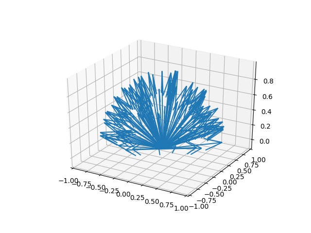
Lastly, we have $\mathscr{R}_{\eta}$ . This is where we enable the use of statistics. In order to have any possibility (or use) for statistical analysis, we need randomness. And this is the term that deals with that. Every time that Alice calculates her next direction to be the average of the directions of her neighbours inside her sphere of influence, $\mathscr{R}_{\eta}$ nudges that trajectory slightly in a random direction. For the purposes of these simulations, we will nudge Alice randomly by a uniformly distributed rotation inside a solid angle $4\pi\eta$ . Uniform distribution simply means that any random rotation is as equally likely as any other. A solid angle on the other hand just defines a slice of a sphere around her new direction that she can be nudged in. The size of the slice is defined by $\eta$ . For example $\eta=0.5$ defines half a sphere. Below you can see what a solid angle of $4\pi\eta$ with $\eta=0.45$ looks like, centred around the north pole (so as if Alice was moving straight up).

This is what a solid angle of $4\pi\eta$ with $\eta=0.45$ centred around the north pole looks like

Well, that's it, right? We've figured out how the equations work, and what they do. What's next? Well, if you remember, what we're trying to achieve here is to add one more thing to the model, to modify it. We need a time delay. We will achieve this very easily. What we can say, is that when Alice is calculating her new trajectory by averaging those of her neighbours, she doesn't take the most current ones, but instead ones from some previous time step. So we simply modify the first equation in the Vicsek model such that

\vec{v_i}(t+1) = v_{0}\mathscr{R}_{\eta}\Theta \left[ \vec{v_i}(t) + \sum_{ j \neq i }{ n_{ij} \vec{v_j}(t-\tau) } \right] ,

and we keep the second one intact

\vec{r_i}(t+1) = \vec{r_i}(t) + \vec{v_i}(t+1) .

All we've done is add a tiny little $\tau$ in the brackets there. This simply states that the velocity vectors of the neighbours will be taken from some previous step $t-\tau$ where $\tau$ can range from $0$ (meaning no time delay), to any number we like. Since in our simulations time will progress in steps of $1$ , $\tau$ can take values like $0, 1, 2, 3...$ .

Cool, now we can proceed to actually

Writing a simulator for the time-delayed Vicsek model in 3D

Now that we've analysed the equations, this will be a very easy task to accomplish. I have two versions of this, one is the one I used for analysing the data written in Python with the help of NumPy (super useful for vector and matrix operations), and the other one to just visualise the model in JavaScript. Let's use the Python code as a reference, since it's more accurate in a couple of aspects.

Another thing to mention, is that we need to set some sort of boundaries to our system, since we can't have them run around in an infinite space. So we will use periodic boundary conditions, which simply means that we will define a box of a certain size, and whenever a particle leaves that box, it will simply reappear on the other end of that box. So, as simple as

if (x < 0):
    x = x + x_size
if (x > x_size):
    x = 0

We also have to be careful about how we calculate distances in periodic boundary conditions . Here's pseudo-code from Wikipedia:

! For a box with the origin at the lower left vertex
! Works for x's lying in any image.
dx = x(j) - x(i)
dx = dx - nint(dx / x_size) * x_size

We also need a function to generate random vectors inside a sphere:

# generate random angle theta between -pi - pi
def rand_vector():
    theta = np.random.uniform(0,2*pi)
    z = np.random.uniform(-1,1)
    x = cos(theta) * sqrt(1 - z**2)
    y = sin(theta) * sqrt(1 - z**2)
    return np.array([x,y,z])

While we are at it, let's also find a way to implement the $\mathscr{R}_{\eta}$ operator. After doing a bit of testing, I found that the fastest way to do this is by using quaternions. These are a mathematical curiosity which allows for algebraic operations with numbers extending the complex numbers. But they have one quite popular use in 3D, and that is calculating rotations.

I've used a dedicated numpy-based library for quaternions, and I've documented my code as much as possible. So we can now put these functions together in one file, and call it geometry3d.py.

geometry3d.py
#!/usr/bin/python
from __future__ import division
import numpy as np
from math import pi, sin, cos, sqrt
from numba import jit
import quaternion as quat

# generate a noise vector inside a cone of angle nu*pi around the north pole
# [1] https://stackoverflow.com/questions/38997302/create-random-unit-vector-inside-a-defined-conical-region
# rotate the generated noise vector to the axis of the particle vector
# [2] https://stackoverflow.com/questions/6802577/rotation-of-3d-vector
def noise_application(noiseWidth, vector):
    
    # Generate a random vector in solid angle 4*pi*nu around north pole
    z = np.random.uniform(0., 1.) * (1 - cos(noiseWidth)) + cos(noiseWidth)
    phi = np.random.uniform(0., 1.) * 2 * np.pi
    x = sqrt(1 - z**2) * cos( phi )
    y = sqrt(1 - z**2) * sin( phi )
    
    # Rotate the noise vector to be in a cone around the directional vector
    # rotation axis
    vector = vector / sqrt(vector[0]**2 + vector[1]**2 + vector[2]**2)
    u =  np.cross([0, 0, 1], vector)
    # rotation angle
    rotTheta = np.arccos(np.dot(vector, [0, 0, 1]))
    # prepare rot angle for quaternion
    axisAngle = 0.5 * rotTheta * u / sqrt(u[0]**2 + u[1]**2 + u[2]**2)
    # Quaternion stuff - pretty fast, compared to rotation matrices
    vec = quat.quaternion(x, y, z)
    qlog = quat.quaternion(*axisAngle)
    q = np.exp(qlog)
    
    vPrime = q * vec * np.conjugate(q)
    
    return vPrime.imag
    
# generate random angle theta between -pi - pi
def rand_vector():
    theta = np.random.uniform(0,2*pi)
    z = np.random.uniform(-1,1)
    x = cos(theta) * sqrt(1 - z**2)
    y = sin(theta) * sqrt(1 - z**2)
    return np.array([x,y,z])

# [3] https://en.wikipedia.org/wiki/Periodic_boundary_conditions#(A)_Restrict_particle_coordinates_to_the_simulation_box
@jit(nopython=True)
def get_all_distances(ps, box_size):
    m = ps.shape[0]
    res = np.zeros((m, m))
    
    for i in range(m):
        for j in range(m):
            dx = abs( ps[i,0] - ps[j,0] )
            dy = abs( ps[i,1] - ps[j,1] )
            dz = abs( ps[i,2] - ps[j,2] )
            dx = dx - np.rint(dx/box_size) * box_size
            dy = dy - np.rint(dy/box_size) * box_size
            dz = dz - np.rint(dz/box_size) * box_size
            res[i, j] = sqrt(dx*dx + dy*dy + dz*dz)
    return res

If you're wondering what's numba and what is that @jit decorator doing there, Numba is a Just In Time compiler for Python, which in short does things real fast, and comparable to C in speed. Go read about it to learn more about it, totally worth it for doing repetitive heavy computations in Python (I measured 7-11x increase in speed in certain scenarios).

Now let's look into simulating the model itself. After we import whatever we will use, we need to declare some variables, which we have in the equations

#!/usr/bin/python
import sys
import numpy as np
from collections import deque
from geometry3d import rand_vector, get_all_distances, noise_application
import time

"""Simulation Variables"""
# Set these before running!!!
# number of particles
N = int(sys.argv[1])

# size of system
box_size = float(sys.argv[2])

# length of time delay
timeDelay = int(sys.argv[3])

# noise intensity
eta = 0.45

# make noise equilibration
noiseWidth = eta*np.pi

# neighbour radius
r = 1.

# time step
t = 0
delta_t = 1

# maximum time steps
T = 20000*delta_t

# velocity of particles
vel = 0.05

"""END Sim Vars"""

We need sys imported, in order to get the arguments passed when running the python script. Now we generate random positions for our particles, and we can use our random vector generator function to initialise random initial velocities for the particles (as well as just initialise an array of zeros for the noise vectors).

"""INITIALISE"""

# initialise random particle positions
particles = np.random.uniform(0,box_size,size=(N,3))
updatePos = particles
prevPos = np.zeros(particles.shape)

# initialise random unit vectors in 3D
rand_vecs = np.zeros((N,3))
for i in range(0,N):
    vec = rand_vector()
    rand_vecs[i,:] = vec
    
noiseVecs = np.zeros((N, 3))
updateVecs = rand_vecs

Finally, we are going to use a queue for the time delay. A way to set this up, is to store in an array the average direction of a particles neighbours, and push it onto a queue. When the queue is filled with $\tau$ values of this average direction, we can dequeue that value, and use it to calculate the next direction of the particle of interest.

# init time delay
updtQueue = np.zeros((N), dtype=deque)
for i in range(N):
    updtQueue[i] = deque()
"""END INIT"""

Next, let's set up the meat of it all - the timestep function, which will do the following for each particle:

Find its neighbours (particles within the sphere of influence)
Put the directions of all neighbours into the queue
When the queue is as long as the time-delay value $\tau$ :
1. Dequeue the neighbours from before the time-delay period
2. Calculate the average direction of the neighbours (and normalise that vector)
3. Apply random noise to that average direction
4. Assign this new vector as the new direction of the particle
5. Move the particle to its new position, following its new direction vector
6. Apply a periodic boundary conditions check (teleport particle if need be)
Rinse and repeat for the duration of the simulation

And then we can add some code to save our particles data to text files, and print in the console the time it takes to make a time step. After all of that, we put everythin in one file, and call it whatever we want, like main.py.

main.py
#!/usr/bin/python
import sys
import numpy as np
from collections import deque
from geometry3d import rand_vector, get_all_distances, noise_application
import time

"""INITIALISE"""

"""Simulation Variables"""
# Set these before running!!!
# number of particles
N = int(sys.argv[1])

# size of system
box_size = float(sys.argv[2])

# length of time delay
timeDelay = int(sys.argv[3])

# noise intensity
eta = 0.45

# neighbour radius
r = 1.

# time step
t = 0
delta_t = 1

# maximum time steps
T = 20000*delta_t

# velocity of particles
vel = 0.05

"""END Sim Vars"""

# make noise equilibration
noiseWidth = eta*np.pi

# initialise random particle positions
particles = np.random.uniform(0,box_size,size=(N,3))
updatePos = particles
prevPos = np.zeros(particles.shape)

# initialise random unit vectors in 3D
rand_vecs = np.zeros((N,3))
for i in range(0,N):
    vec = rand_vector()
    rand_vecs[i,:] = vec
    
noiseVecs = np.zeros((N, 3))
updateVecs = rand_vecs

timestepTime = time.time()

# init time delay
updtQueue = np.zeros((N), dtype=deque)
for i in range(N):
    updtQueue[i] = deque()
"""END INIT"""

def timestep(particles, rand_vecs):
    
    # actual simulation timestep
    for i in range(len(particles)):
        
        # get neighbor indices for current particle
        neighbours = np.where(distances[i]<r)
        neighbours = neighbours[0][ np.where( neighbours[0] != i ) ]
        
        neighsDirs = rand_vecs[neighbours]
        
        # add neighbours' directions to queue to be used after time delay interval
        updtQueue[i].append(neighsDirs)
        
        # if the queue is long enough, dequeue and change unit vector accordingly
        # otherwise continue on previous trajectory
        if(len(updtQueue[i]) > timeDelay):
            
            # get neighbours' directions from before time delay interval
            neighsDirs = updtQueue[i].popleft()
            
            # get average direction vector of neighbours
            avg = np.mean([rand_vecs[i], *neighsDirs], axis=0)
            
            # apply the noise vector by rotating it to the axis of the particle vector
            newVec = noise_application(noiseWidth, avg)
            
            # move to new position 
            updatePos[i,:] = updatePos[i,:] + delta_t * vel * newVec
            
            # get new unit vector vector
            updateVecs[i] = newVec
        else:
            # move to new position using old unit vector
            updatePos[i,:] = updatePos[i,:] + delta_t * vel * rand_vecs[i]
    
        # assure correct boundaries (xmax,ymax) = (box_size, box_size)
        if updatePos[i,0] < 0:
            updatePos[i,0] = box_size + updatePos[i,0]
    
        if updatePos[i,0] > box_size:
            updatePos[i,0] = updatePos[i,0] - box_size
    
        if updatePos[i,1] < 0:
            updatePos[i,1] = box_size + updatePos[i,1]
    
        if updatePos[i,1] > box_size:
            updatePos[i,1] = updatePos[i,1] - box_size
    
        if updatePos[i,2] < 0:
            updatePos[i,2] = box_size + updatePos[i,2]
    
        if updatePos[i,2] > box_size:
            updatePos[i,2] = updatePos[i,2] - box_size
            
    particles = updatePos
    rand_vecs = updateVecs
    
    return particles, rand_vecs

"""TIMESTEP AND THINGS TO DO WHEN VISITING"""    
# Run until time ends
timestr = time.strftime("%Y%m%d-%H%M%S")
f = open( 'N{0}L{1}dt{2}T{3}_{4}.txt'.format(N, box_size, timeDelay, T, timestr), 'a+' )
while t < T:
    # print progress update and time spent on n steps
    if t%100 == 0:
        print ("step {} / {}: avg. time for 10 steps {:.3f}".format(
                t, T, (time.time()-timestepTime)/10
                ))
        timestepTime = time.time()
        
    """Timestep"""
    
    # get all relative distances between particles before looking for neighbours
    distances = get_all_distances(particles, box_size)
    
    particles, rand_vecs = timestep(particles, rand_vecs)
    
    # export data and advance to new time step
    np.savetxt(f, particles, header='timestep {0}'.format(t) )
    t += delta_t
    
else:
    f.close()

And we are done! We can now run our simulator from the terminal with something like python main.py 128 6 2 to get the simulation for 128 particles, a box size of 6, and time delay value of 2. Voila! We have a Vicsek model simulator with added time delay, which will export particle positions. Now we can do all kinds of fun things, like visualise the motion of the particles, or do analysis on the data.

Next time we will see what kind of statistical analysis we can do on those data, and for now I will leave you with a link to a visualisation version of this model, that you can play around with

And here you can see the full code of the simulator, together with the analysis part, and a script to run it, as well as a Jupyter notebook for visualising the analysis. We will discuss all of these in the next post.

Thank you for reading!

The information in this blog, as well as all the tools, apps and libraries I develop are currently open source.

I would love to keep it this way, and you can help!

You can buy me a coffee from here, which will go towards the next all-nighter I pull off!

Or you can support me and my code monthly over at Github Sponsors!

Thanks!

Analysing the equations of motion​

Writing a simulator for the time-delayed Vicsek model in 3D​

Analysing the equations of motion

Writing a simulator for the time-delayed Vicsek model in 3D